Spreadsheets are some of my favorite things. I know that was super nerdy, but what else would you expect from me? As someone who likes organization, automation, and data calculations, I really enjoy the power I experience from using formulas that help me to do just that! So, here are 4 of my favorite Google Sheets formulas that make me feel like a super hero!
=IMPORTRANGE
This formula is truly one of my favorites. I use this formula a lot to pull data from one spreadsheet into a totally different spreadsheet. Why would I want to use this, you ask? Let me give you an example. Suppose you have some amazing data in a massive multi-tab spreadsheet in Google Sheets. But, rather than sharing the entire spreadsheet with someone, you want to only share the data in one particular tab. You could always copy and paste that data into a new spreadsheet, but if the master data set is a work in progress, you will want some way to give that person constant access to the current set. I present to you the Import Range formula!
Import Range takes the data range in that tab, sends it to your new spreadsheet, and constantly updates the data in the new spreadsheet as it changes in the master spreadsheet. So, here’s the formula:
=importrange("SpreadsheetURL","’Tab Name’!Range of Data to Import")
In the example below, I’m importing data from this spreadsheet “docs.google.com/spreadsheet/12345” and I want to Import all data in the tab named “List1” that has data in Column A - Column E.
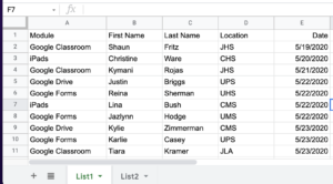
In my new spreadsheet I’ll use this formula in the first cell of the sheet:
=importrange(“docs.google.com/spreadsheet/12345”, “List1!A:F”)
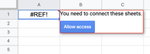
I have to then give permission to use the data in my master spreadsheet from a popup that appears in the cell.
Viola, I have imported my data set!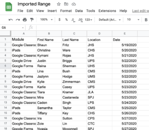
=FILTER
Now, for that spreadsheet containing the data I have imported, let’s say I want to create a new tab that contains an automatically filtered listing of people who have completed a particular module. I can use filter views, but that often means I have to keep turning filters on and off. There has to be an easier way, and there is, it’s the FILTER formula!
=filter(‘Tab Name’!DataRange,’Tab Name’!FirstSearchLocation:Condition")
I have the sheet of data that I want to Filter by the Module each person completed. I created a new tab called “Google Classroom Only” where I will be working.
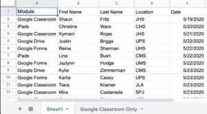
I will use the following formula in the new tab.
=FILTER(Sheet1!A2:E,Sheet1!A2:A="Google Classroom")
(Note: I tell the formula to start at the first true entry to search, A2. If you use A:E rather than A2:E, you will get an error message regarding range size mismatches.)
I now have a filtered listing of only those who completed the Google Classroom Module.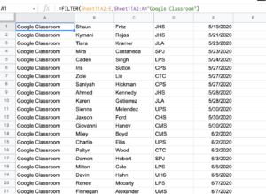
I can now use the same technique to make a new tab for each module to better organize the data.
=LEFT & =RIGHT
These awesome formulas allow you to truncate data after a certain number of characters starting either from the LEFT or the RIGHT side of the cell. The formula looks like this:
=LEFT(Cell, Number of characters to keep)
=RIGHT(Cell, Number of characters to keep)
In my data set I’ve been using, let’s say I want only the first initial of everyone’s first name.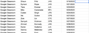
Since I’d be starting on the left, I’ll use the LEFT formula. I’ll start with cell B1 and tell it to only keep one character:
=LEFT(B1, 1)![]()
Once I get the desired result, I copy and paste that formula down the column to have it match up with the associated rows.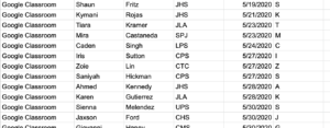
=LOWER & =UPPER
Sometimes I need to remove the capitalization of words or names, especially in cases of assumed usernames. The Lower and Upper formulas allow me to do just that:
=LOWER(Cell)
=UPPER(Cell)
In my data set, I want a column of all of the first initials as lowercase letters and a column of all of the last names in lowercase. To do this, I’ll use the Lower formula twice.
I’ll start in cell F1 since that’s where my initials begin. I’ll use this formula in the Cell G1:
Now I can copy and paste both formulas down the columns to get my lowercase versions of the data.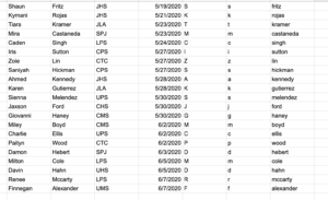
Spreadsheets are amazing and can make you feel extremely powerful when it comes to organizing your data. You can check out some other awesome spreadsheet formulas for Google Sheets on the Google Sheets Function List.
Written by Daniel Vanover. Daniel is a Technology Coach for Wise County Public Schools and is a Google Certified Educator, Trainer, and Administrator. You can connect with him and get more information on his website.
